What does AUC stand for and what is it?
A note to clarify the defination
What does AUC stand for and what is it?
For classification machine learning model, it’s unwise to use Accuracy as single measurement for model performance, most of the time, we use AUC (Area Under the Curve) and Confusion Matrix, F1 score as a combination measurement to justify the performance of a classficiation machine learning model, but what exactly is AUC, what exactly is Area and the Curve? I wanna to take a note for future reference.
Abbreviations
- AUC = Area Under the Curve
- AUROC = Area Under the Receiver Operating Characteristic Curve.
AUC is used most of the time mean AUROC, which is bad practice since as Marc Claesen pointed out AUC is ambiguous (could be any curve) while AUROC is not.
Interpreting the AUROC
The AUROC has several equivalent interpretations
- The expectation that a uniformly drawn random positive is ranked before a uniformly drawn random negative.
- The expected proportion of positives ranked before a uniformly drawn random negative.
- The expected true positive rate if the ranking is split just before a uniformly drawn random negative.
- The expected proportion of negatives ranked after a uniformly drawn random positive.
- The expected false positive rate if the ranking is split just after a uniformly drawn random positive.
Going further: How to derive the probabilistic interpretation of the AUROC?
Computing the AUROC
Assume we have a probabilistic, binary classifier such as logistic regression.
Before presenting the ROC curve (= Receiver Operating Characteristic curve), the concept of confusion matrix must be understood. When we make a binary prediction, there can be 4 types of outcomes:
- We predict 0 while the true class is actually 0: this is called a True Negative, i.e. we correctly predict that the class is negative (0). For example, an antivirus did not detect a harmless file as a virus.
- We predict 0 while the true class is actually 1: this is called a False Negative, i.e. we incorrectly predict that the class is negative (0). For example, an antivirus failed to detect a virus.
- We predict 1 while the true class is actually 0: this is called a False Positive, i.e. we incorrectly predict that the class is positive (1). For example, an antivirus considered a harmless file to be a virus.
- We predict 1 while the true class is actually 1: this is called a True Positive, i.e. we correctly predict that the class is positive (1). For example, an antivirus rightfully detected a virus.
To get the confusion matrix, we go over all the predictions made by the model, and count how many times each of those 4 types of outcomes occur:
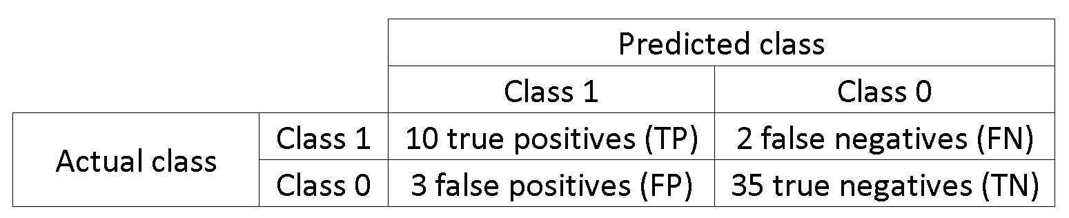
In this example of a confusion matrix, among the 50 data points that are classified, 45 are correctly classified and the 5 are misclassified.
Since to compare two different models it is often more convenient to have a single metric rather than several ones, we compute two metrics from the confusion matrix, which we will later combine into one:
-
True Positive Rate, aka. Sensitivity, Hit Rate or Recall Rate, which defined as $\frac{TP}{TP+FN}$. Intuitively this metric corresponds to the proportion of positive data points that are correctly considered as positive, with respect to all positive data points. In other words, the higher True Positive Rate, the fewer positive data points we will miss.
-
False Positive Rate, aka fall-out, which is defined as $\frac{FP}{FP+TN}$. Intuitively this metric corresponds to the proportion of negative data points that are mistakenly considered as positive, with respect to all negative data points. In other words, the higher False Positive Rate, the more negative data points will be missclassified.
To combine the False Positive Rate and the True Positive Rate into one single metric, we first compute the two former metrics with many different threshold (for example 0.00, 0.01, 0.02, ..., 1.00) for the logistic regression, then plot them on a single graph, with the False Positive Rate values on the abscissa and the True Positive Rate values on the ordinate. The resulting curve is called ROC curve, and the metric we consider is the AUC of this curve, which we call AUROC.
The following figure shows the AUROC graphically:
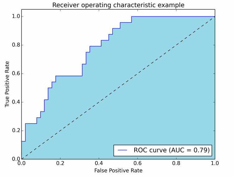
In this figure, the blue area corresponds to the Area Under the curve of the Receiver Operating Characteristic (AUROC). The dashed line in the diagonal we present the ROC curve of a random predictor: it has an AUROC of 0.5. The random predictor is commonly used as a baseline to see whether the model is useful.
If you want to get some first-hand experience: